Browse By Unit
4.6 Approximating Values of a Function Using Local Linearity and Linearization
1 min read•june 18, 2024
4.6 Approximating Values of a Function Using Local Linearity and Linear
Imagine you're hiking up a winding mountain trail. At any given point on the trail, the path might seem pretty straight, right? That path is your tangent line, which is like a snapshot of the trail’s behavior at that specific point. In this topic, we’ll see how we can use this straight tangent line to approximate values of not-so-straight functions. ⭐
↗️ Linearization and Tangent Line Approximation
Recall back from Unit 2 and our discussion of the definition of the derivative and tangent lines. At any one point, the slope of the line tangent to the graph is the function’s derivative at that single point. Using this slope and the coordinates of your point, you can construct an equation for the tangent line using the point-slope formula, which is as follows:
While you might come across a different-looking formula for linearization, it is essentially the same as the point-slope formula. If you’d like to memorize yet another formula for this exam, you can absolutely do so! However, using the point-slope formula is an easier fail-safe to fall back on for the AP Exam. Here is the linearization formula:
Once you have both your x and y points as well as the slope of your tangent line, you’re ready to approximate! Using your constructed tangent line formula, plug in the x-value you want to estimate and solve for y. This will give you your approximation. Wasn’t that easy?
🔀 Under / Overestimations
On the AP Calculus exam, they love to ask you to determine whether or not your estimations are greater or less than the actual value. Luckily, we can make out if our linear approximation was an overestimate or underestimate by observing the behavior of the function at the point of tangency.
If at the point of tangency, the graph is concave up, then we can assume our linearization is an underestimate. This is because the whole tangent line will always be under the curve, making every value less than the actual function value.
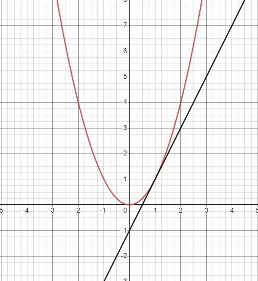
Graph created with Desmos
If at the point of tangency, the graph is concave down, then we can assume our linearization is an overestimate. The opposite holds true here. Since the whole tangent line is always above the curve, every value is greater than the actual function value.
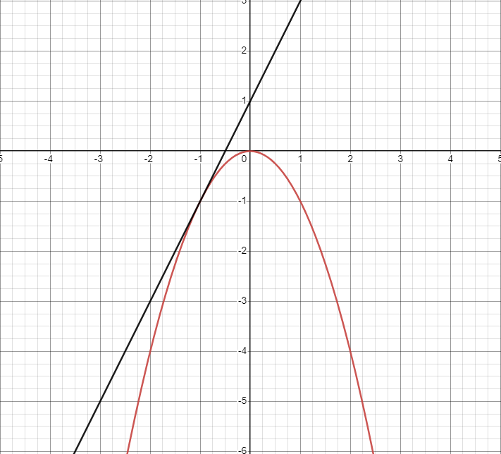
Graph created with Desmos
Linearization Practice Questions
The following free-response question (FRQ) is from the 2010 AP Calculus AB examination administered by College Board. All credit to College Board.
Solutions to the differential equation also satisfy Let be a particular solution to the differential equation with
2010 AP Calculus AB #6a
a) Write an equation for the line tangent to the graph of at x = 1.
To start this question, we must first find the slope of our tangent line at the point x = 1. Because we have the point (1,2) given in the problem, all we have to do is plug it into the derivative:
Using this, we can now plug everything into our point-slope form to get our tangent line equation:
2010 AP Calculus AB #6b
b) Use the tangent line equation from part (a) to approximate . Given that for , is the approximation for greater than or less than ? Explain your reasoning.
Now that we have our tangent line equation, we can use it to estimate a point on our function. Using the equation and plugging in , we get:
Because we’re given that for , we know that the function is concave up, or its second derivative is greater than 0. So, this means our approximation has to be an underestimate, as it is lower than the point on the function. Awesome work! 🤗
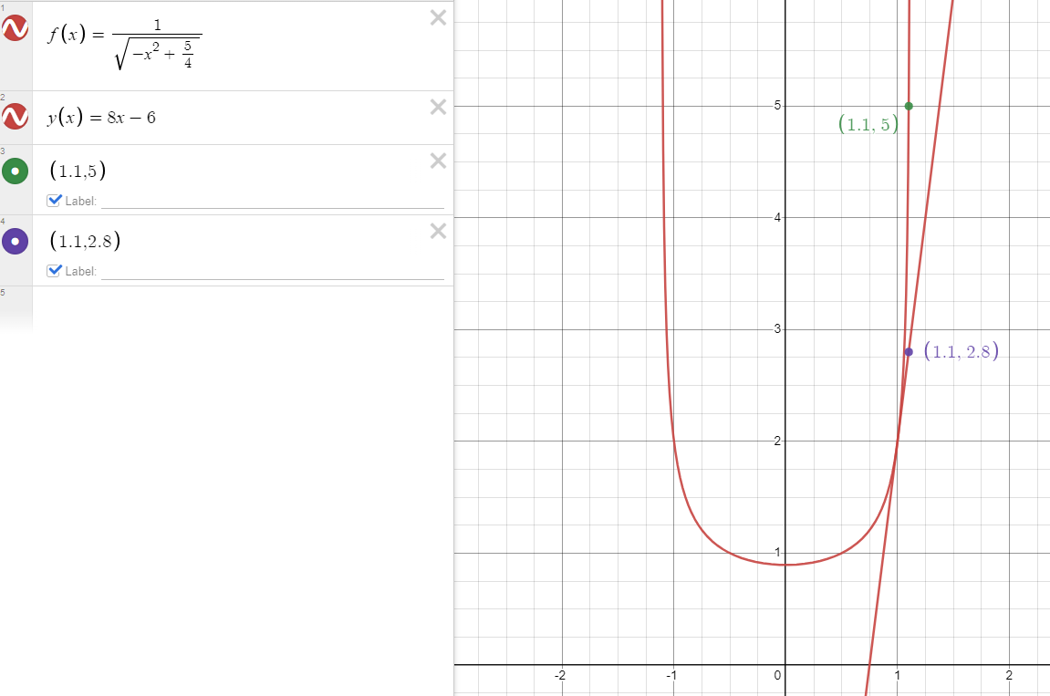
Graph created with Desmos
🔷 Closing
Nice work!! 🙌
You are now able to construct and use tangent lines to approximate a point on a function, as well as determine whether this approximation is an overestimation or underestimation. While this skill may be simpler than others you’ll learn, it is still very important to refine and remember for the AP exam in May. Have fun practicing!
<< Hide Menu
4.6 Approximating Values of a Function Using Local Linearity and Linearization
1 min read•june 18, 2024
4.6 Approximating Values of a Function Using Local Linearity and Linear
Imagine you're hiking up a winding mountain trail. At any given point on the trail, the path might seem pretty straight, right? That path is your tangent line, which is like a snapshot of the trail’s behavior at that specific point. In this topic, we’ll see how we can use this straight tangent line to approximate values of not-so-straight functions. ⭐
↗️ Linearization and Tangent Line Approximation
Recall back from Unit 2 and our discussion of the definition of the derivative and tangent lines. At any one point, the slope of the line tangent to the graph is the function’s derivative at that single point. Using this slope and the coordinates of your point, you can construct an equation for the tangent line using the point-slope formula, which is as follows:
While you might come across a different-looking formula for linearization, it is essentially the same as the point-slope formula. If you’d like to memorize yet another formula for this exam, you can absolutely do so! However, using the point-slope formula is an easier fail-safe to fall back on for the AP Exam. Here is the linearization formula:
Once you have both your x and y points as well as the slope of your tangent line, you’re ready to approximate! Using your constructed tangent line formula, plug in the x-value you want to estimate and solve for y. This will give you your approximation. Wasn’t that easy?
🔀 Under / Overestimations
On the AP Calculus exam, they love to ask you to determine whether or not your estimations are greater or less than the actual value. Luckily, we can make out if our linear approximation was an overestimate or underestimate by observing the behavior of the function at the point of tangency.
If at the point of tangency, the graph is concave up, then we can assume our linearization is an underestimate. This is because the whole tangent line will always be under the curve, making every value less than the actual function value.

Graph created with Desmos
If at the point of tangency, the graph is concave down, then we can assume our linearization is an overestimate. The opposite holds true here. Since the whole tangent line is always above the curve, every value is greater than the actual function value.

Graph created with Desmos
Linearization Practice Questions
The following free-response question (FRQ) is from the 2010 AP Calculus AB examination administered by College Board. All credit to College Board.
Solutions to the differential equation also satisfy Let be a particular solution to the differential equation with
2010 AP Calculus AB #6a
a) Write an equation for the line tangent to the graph of at x = 1.
To start this question, we must first find the slope of our tangent line at the point x = 1. Because we have the point (1,2) given in the problem, all we have to do is plug it into the derivative:
Using this, we can now plug everything into our point-slope form to get our tangent line equation:
2010 AP Calculus AB #6b
b) Use the tangent line equation from part (a) to approximate . Given that for , is the approximation for greater than or less than ? Explain your reasoning.
Now that we have our tangent line equation, we can use it to estimate a point on our function. Using the equation and plugging in , we get:
Because we’re given that for , we know that the function is concave up, or its second derivative is greater than 0. So, this means our approximation has to be an underestimate, as it is lower than the point on the function. Awesome work! 🤗

Graph created with Desmos
🔷 Closing
Nice work!! 🙌
You are now able to construct and use tangent lines to approximate a point on a function, as well as determine whether this approximation is an overestimation or underestimation. While this skill may be simpler than others you’ll learn, it is still very important to refine and remember for the AP exam in May. Have fun practicing!

© 2025 Fiveable Inc. All rights reserved.