Browse By Unit
5.9 Connecting a Function, Its First Derivative, and its Second Derivative
6 min read•february 15, 2024
Beth
Beth
In previous guides, we learned all about making conclusions regarding the behavior of a function based on the behavior of its derivatives such as whether the function is increasing or decreasing at a point, concave up or concave at a point, and more! While we mostly focused on algebraically determining the behavior of functions, we can also determine information graphically! The key features of the graphs of , , and are all related to one another. 🔑
Let’s dive into how we can do that!
📈 Connecting a Function, Its First Derivative, and Its Second Derivative
Given the graphs of , , and or some combination of the three, we can determine information about another much as we did so algebraically. The knowledge you learned in our previous Unit 5 subtopic guides can be carried over to this subtopic—instead of using the equations for , , and , you can look at (one of) their graphs and see where the -axis is crossed or where the graph is positive or negative, increasing or decreasing, etc, to infer information about the other graphs.
📉 Trends and Concavity
Here’s a quick summary of what you’ve learned so far in this unit about trends and concavity:
- When a function is increasing, the first derivative will be positive ().
- When a function is decreasing, the first derivative will be negative ().
- When a function is concave up, the second derivative will be positive () and the first derivative will increase.
- When a function is concave down, the second derivative will be negative () and the first derivative will decrease.
👀 Trends and Concavity Graphically
Let’s apply this information to the following graph of a function, .
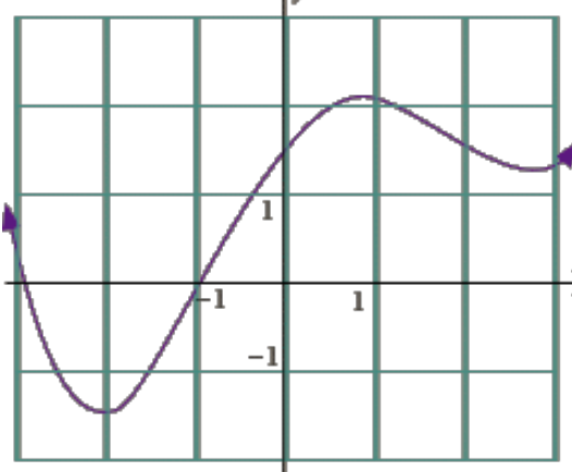
Image Courtesy of Zweig Media
Taking a look at this graph, we can describe between each interval:
- From and , is decreasing, so is negative.
- From and , is increasing, so is positive.
What about ? Let’s take a look at the concavity of :
- From and , is concave up. Therefore, is positive and is increasing.
- From , is concave down. Therefore, is negative and is decreasing.
🔍 Extrema and Points of Inflection
Based on where the graph of the function changes direction and concavity, we can also interpret maximums, minimums, x-intercepts, and points of inflection of the graphs of the first and second derivatives.
- If has a relative minimum (the graph changes from decreasing to increasing), then will change from negative to positive at that point.
- If has a relative maximum (the graph changes from increasing to decreasing), then will change from positive to negative at that point.
- If has a point of inflection, changing from concave up to concave down, then will have a relative maximum and will change from positive to negative at that point.
- If has a point of inflection, changing from concave down to concave up, then will have a relative minimum and will change from negative to positive at that point.
If we boil this down to two key concepts, realize that:
- All relative extrema of are x-intercepts of .
- All points of inflection of are relative extrema of .
This may seem like a lot, but once you see it in action, it’ll make more sense! ⬇️
👀 Extrema and POIs Graphically 1
Here’s a relatively easy example! The derivative of the differentiable function , , is graphed.
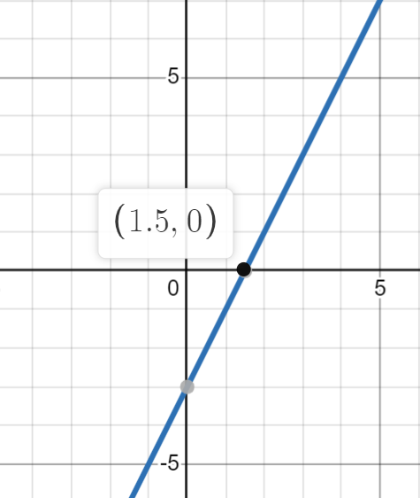
Image Created with Desmos.
What can we tell about at the point based on the graph of its derivative ?
By looking at the graph of , we see that crosses the x-axis at the point of interest . It is negative before and positive after . This means that is decreasing before the point and increasing after it, indicating that the point is a relative minimum on the graph of .
The justification we used above to determine the answer is essentially just applying the First Derivative Test but in graphical form! Here’s a quick look at and so you can really see their relationship:
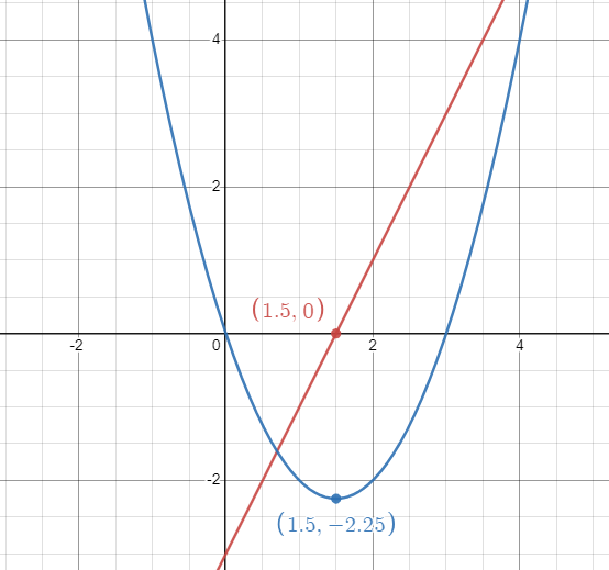
Image Created with Desmos.
👀 Extrema and POIs Graphically 2
Now, let’s take another look at the example before, but focus on relative extrema and points of inflection.

Image Courtesy of Zweig Media.
You’ll notice the following:
- At and , has relative minima. Therefore, has x-intercepts at these points and will change from negative to positive.
- At , has a relative maximum. has another x-intercept, but the opposite is true: will change from positive to negative.
- At , has a point of inflection, changing from concave up to concave down. This means will have a relative maximum and has an x-intercept changing from positive to negative at .
- At , has an inflection point, but it changes from concave down to concave up. Therefore, has a relative minimum and has an x-intercept changing from negative to positive at .
👀 Extrema and POIs Graphically 3
Before you move on to taking a look at graphs yourself, take a look at the following graph of and think about:
- What happens to at , denoted by the red dotted line?
- What happens to at , denoted by the black dotted line?
- What happens to at ?
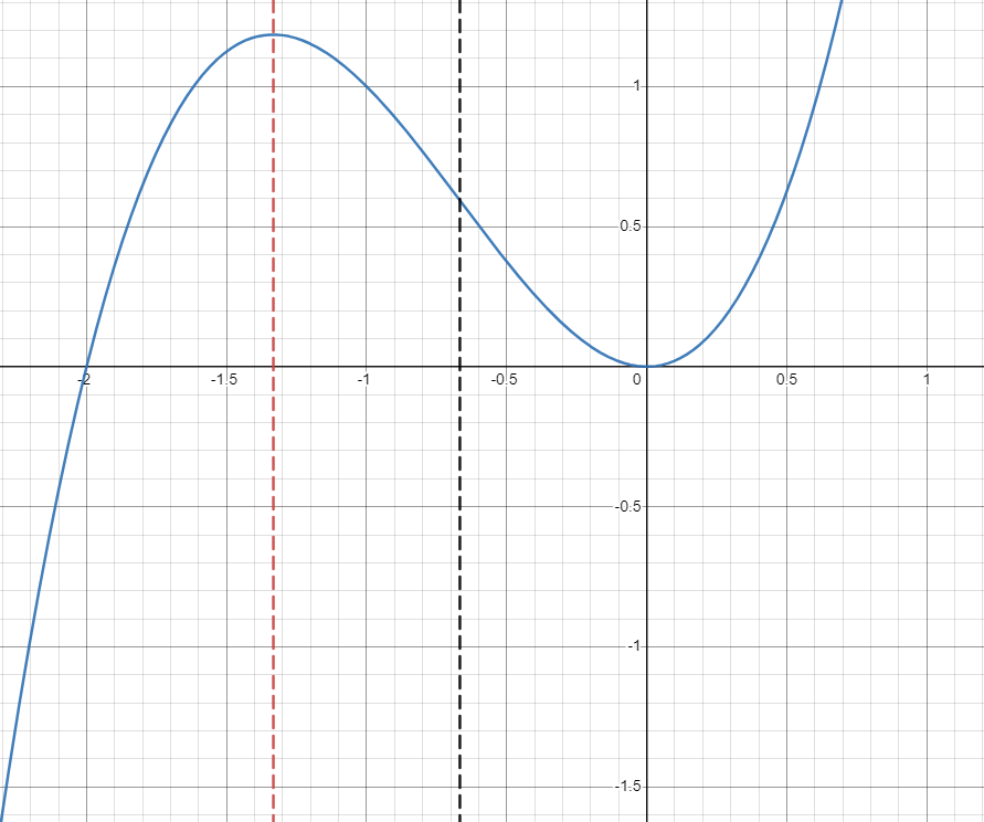
Image Created with Desmos.
At , has a relative maximum. This tells us that will have an x-intercept at this point and change from positive to negative!
At , changes from being concave down to concave up. This tells us that will have a relative minimum at this point and has an x-intercept, changing from negative to positive.
Take a look at in blue and in green! You can see exactly these trends.
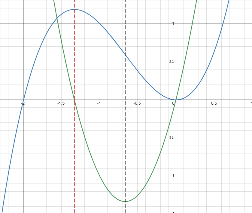
Image Created with Desmos.
And here’s a graph with added as well, denoted in purple.
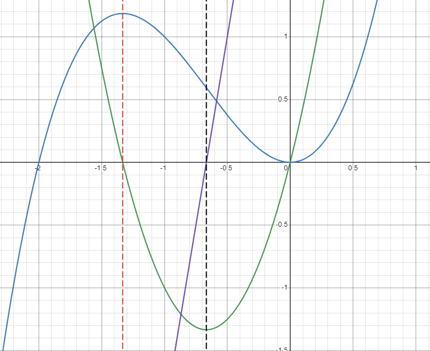
Image Created with Desmos.
📝Practice Problems
Now it’s time for you to do some practice on your own! These won’t be as tough, they will more generally test your knowledge of these trends.
❓Practice Problems
Question 1:
The second derivative of the differentiable function , , is graphed.
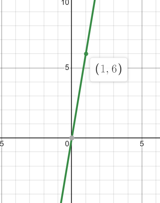
Image Created with Desmos.
Given that , what can we tell about at the point based on the graph of its second derivative ?
Question 2:
The second derivative of the differentiable function , , is graphed.
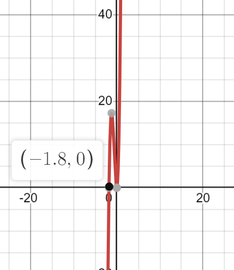
Image Created with Desmos.
What can we tell about at the point based on the graph of its second derivative ?
✅ Answers and Solutions
Question 1:
Answer: has a relative minimum at the point .
Solution:
By looking at the graph of , we see that is positive at the point of interest . This means that is concave up at the point. Combined with the fact that , we can apply the Second Derivative Test to conclude that has a minimum at .
Question 2:
Answer: is concave down at the point .
Solution:
By looking at the graph of , we infer that is negative at the point of interest . This means that is concave down at the point.
⭐ Closing
Woah! You made it to the end of this guide. To practice with some of this material, we recommend getting into Desmos and graphing a function, its first derivative, and its second derivative to see the features of each. Good luck! 🍀
<< Hide Menu
5.9 Connecting a Function, Its First Derivative, and its Second Derivative
6 min read•february 15, 2024
Beth
Beth
In previous guides, we learned all about making conclusions regarding the behavior of a function based on the behavior of its derivatives such as whether the function is increasing or decreasing at a point, concave up or concave at a point, and more! While we mostly focused on algebraically determining the behavior of functions, we can also determine information graphically! The key features of the graphs of , , and are all related to one another. 🔑
Let’s dive into how we can do that!
📈 Connecting a Function, Its First Derivative, and Its Second Derivative
Given the graphs of , , and or some combination of the three, we can determine information about another much as we did so algebraically. The knowledge you learned in our previous Unit 5 subtopic guides can be carried over to this subtopic—instead of using the equations for , , and , you can look at (one of) their graphs and see where the -axis is crossed or where the graph is positive or negative, increasing or decreasing, etc, to infer information about the other graphs.
📉 Trends and Concavity
Here’s a quick summary of what you’ve learned so far in this unit about trends and concavity:
- When a function is increasing, the first derivative will be positive ().
- When a function is decreasing, the first derivative will be negative ().
- When a function is concave up, the second derivative will be positive () and the first derivative will increase.
- When a function is concave down, the second derivative will be negative () and the first derivative will decrease.
👀 Trends and Concavity Graphically
Let’s apply this information to the following graph of a function, .

Image Courtesy of Zweig Media
Taking a look at this graph, we can describe between each interval:
- From and , is decreasing, so is negative.
- From and , is increasing, so is positive.
What about ? Let’s take a look at the concavity of :
- From and , is concave up. Therefore, is positive and is increasing.
- From , is concave down. Therefore, is negative and is decreasing.
🔍 Extrema and Points of Inflection
Based on where the graph of the function changes direction and concavity, we can also interpret maximums, minimums, x-intercepts, and points of inflection of the graphs of the first and second derivatives.
- If has a relative minimum (the graph changes from decreasing to increasing), then will change from negative to positive at that point.
- If has a relative maximum (the graph changes from increasing to decreasing), then will change from positive to negative at that point.
- If has a point of inflection, changing from concave up to concave down, then will have a relative maximum and will change from positive to negative at that point.
- If has a point of inflection, changing from concave down to concave up, then will have a relative minimum and will change from negative to positive at that point.
If we boil this down to two key concepts, realize that:
- All relative extrema of are x-intercepts of .
- All points of inflection of are relative extrema of .
This may seem like a lot, but once you see it in action, it’ll make more sense! ⬇️
👀 Extrema and POIs Graphically 1
Here’s a relatively easy example! The derivative of the differentiable function , , is graphed.

Image Created with Desmos.
What can we tell about at the point based on the graph of its derivative ?
By looking at the graph of , we see that crosses the x-axis at the point of interest . It is negative before and positive after . This means that is decreasing before the point and increasing after it, indicating that the point is a relative minimum on the graph of .
The justification we used above to determine the answer is essentially just applying the First Derivative Test but in graphical form! Here’s a quick look at and so you can really see their relationship:

Image Created with Desmos.
👀 Extrema and POIs Graphically 2
Now, let’s take another look at the example before, but focus on relative extrema and points of inflection.

Image Courtesy of Zweig Media.
You’ll notice the following:
- At and , has relative minima. Therefore, has x-intercepts at these points and will change from negative to positive.
- At , has a relative maximum. has another x-intercept, but the opposite is true: will change from positive to negative.
- At , has a point of inflection, changing from concave up to concave down. This means will have a relative maximum and has an x-intercept changing from positive to negative at .
- At , has an inflection point, but it changes from concave down to concave up. Therefore, has a relative minimum and has an x-intercept changing from negative to positive at .
👀 Extrema and POIs Graphically 3
Before you move on to taking a look at graphs yourself, take a look at the following graph of and think about:
- What happens to at , denoted by the red dotted line?
- What happens to at , denoted by the black dotted line?
- What happens to at ?

Image Created with Desmos.
At , has a relative maximum. This tells us that will have an x-intercept at this point and change from positive to negative!
At , changes from being concave down to concave up. This tells us that will have a relative minimum at this point and has an x-intercept, changing from negative to positive.
Take a look at in blue and in green! You can see exactly these trends.

Image Created with Desmos.
And here’s a graph with added as well, denoted in purple.

Image Created with Desmos.
📝Practice Problems
Now it’s time for you to do some practice on your own! These won’t be as tough, they will more generally test your knowledge of these trends.
❓Practice Problems
Question 1:
The second derivative of the differentiable function , , is graphed.

Image Created with Desmos.
Given that , what can we tell about at the point based on the graph of its second derivative ?
Question 2:
The second derivative of the differentiable function , , is graphed.

Image Created with Desmos.
What can we tell about at the point based on the graph of its second derivative ?
✅ Answers and Solutions
Question 1:
Answer: has a relative minimum at the point .
Solution:
By looking at the graph of , we see that is positive at the point of interest . This means that is concave up at the point. Combined with the fact that , we can apply the Second Derivative Test to conclude that has a minimum at .
Question 2:
Answer: is concave down at the point .
Solution:
By looking at the graph of , we infer that is negative at the point of interest . This means that is concave down at the point.
⭐ Closing
Woah! You made it to the end of this guide. To practice with some of this material, we recommend getting into Desmos and graphing a function, its first derivative, and its second derivative to see the features of each. Good luck! 🍀

© 2025 Fiveable Inc. All rights reserved.