Browse By Unit
6.1 Integration and Accumulation of Change
4 min read•june 18, 2024
Emery
Emery
Untitled
Onto unit 6 of AP Calculus! If you were asked to calculate how many miles a car traveled in 3 hours moving at a constant speed of 65 miles per hour, how would you do it? Using this example, you’ll learn about Riemann sums, the basics of integral calculus, and how to apply it to real life!
🏎️ Change Over Time
Accumulation of change is exactly what it sounds like—the sum, over time, of how much something has changed. Let’s return to the example at the beginning: we want to know how far a car has traveled, and we are given its speed (in miles per hour) and the length of time it has been traveling. We want to know how many miles it has accumulated over 3 hours. This problem is fairly straightforward, and we can solve it with a simple equation:
where d is distance, v is velocity (speed), and t is time. Let’s apply it to the problem.
Notice that because we have the unit hours in the denominator of one term and the numerator of the other, they cancel, leaving us with just a unit of miles. This is how units will work for all of these problems—they should be the unit of the rate of change multiplied by the independent variable.
We’ve solved our first problem! Now, let’s connect it to calculus.
📈 Graphing Change Over Time
We can depict the relationship between how fast, how long, and how far the car traveled with a graph.
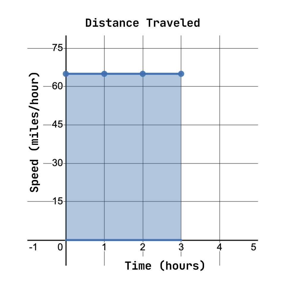
Image courtesy of Emery
Here, we can see that the x-axis represents how long the car has been traveling and the y-axis represents how fast it is traveling. The shaded area under the curve represents the total distance traveled.
This example is about a car that is traveling at a constant speed, as though it was on the highway using cruise control. But in reality, a whole trip for a vehicle involves variation in speed. Let’s look at another example, where a car leaves its house, accelerates to 50 miles per hours, drives on the highway for almost two hours, decelerates to 20 miles per hour, finishes driving to its destination, and then decelerates to 0 miles per hour. How far did the car travel?
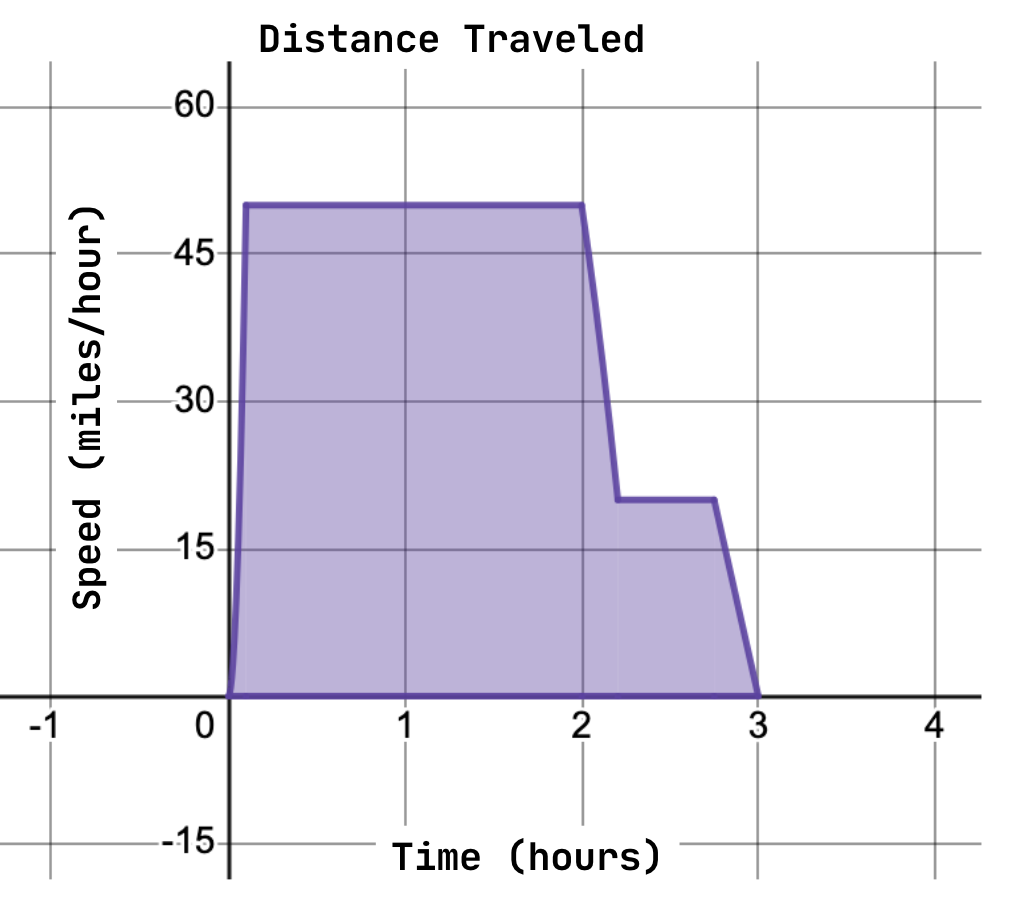
Image courtesy of Emery
Based on our simpler example, we know that the shaded area under the curve will give us the distance the car traveled. But, we can’t just use the equation for an area of a rectangle here, because it’s a much more complex shape! The following piecewise function describes the curve:
There are a few different ways we can approach this problem: by estimating using rectangles, or by using an integral.
📊 Riemann Sums
The first way we can find area under the curve is by using something called a Riemann Sum. This involves drawing rectangles, or other easy shapes to take the area of, and using them to approximate the area under the curve. Let’s apply it to our problem!
✏️ Riemann Sum: Step-by-Step
Step 1: How Many Rectangles?
The first thing we need to do is decide how many rectangles we want to use to approximate our area under the curve. For simplicity’s sake, let’s just use six in this example. We want them to have equal widths, so we divide our total base by our number of rectangles. Since the car’s trip was three hours long, we’ll divide 3 by 6, to find a base length of 0.5. Step 2: Graphing****
Let’s add our six rectangles to our initial graph:
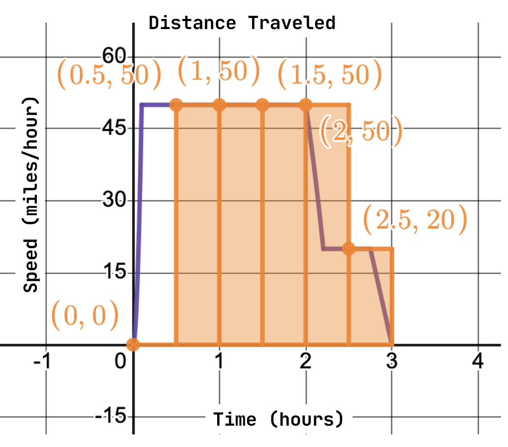
Image courtesy of Emery
Step 3: Computation
Finally, let’s create a table and calculate the area of each rectangle. Our table of values looks like this:
| Base | Height |
| 0.5 | 0 |
| 0.5 | 50 |
| 0.5 | 50 |
| 0.5 | 50 |
| 0.5 | 50 |
| 0.5 | 20 |
To calculate the total area, we will sum the areas of each of these rectangles like so:
Since our base length is the same, we can factor it out and simplify our equation like this:
Therefore, using this simple approximation, we find that our car has traveled about 110 miles! However, based on the graph, we can see that this is probably somewhat inaccurate, as it includes both overestimations and underestimations of the true distance traveled. This is where integrals come in!
📈 Preview of Integrals
So far, we’ve worked on approximating the area under the curve, or the accumulation of change. But, we have a very powerful tool at our disposal—the integral. Integrals are also called anti-derivatives, which is exactly what it sounds like! They “undo” derivation, just like multiplication undoes division. They also calculate the exact area under the curve.
Integration is represented with the following notation:
This notation tells us to find the area under the curve for our function over the interval [0,3]. This type of integral is specifically called a definite integral. We won’t cover how to take the integral right now, but if you did take it, you would find that the exact area under the curve in our example problem is 117.44 miles.
📝 Practice
Let’s look at one final sample problem before trying it on your own!
Example Problem: Consider the following graph of the function , which represents the total distance traveled by a vehicle over time. What is the average speed of the vehicle?
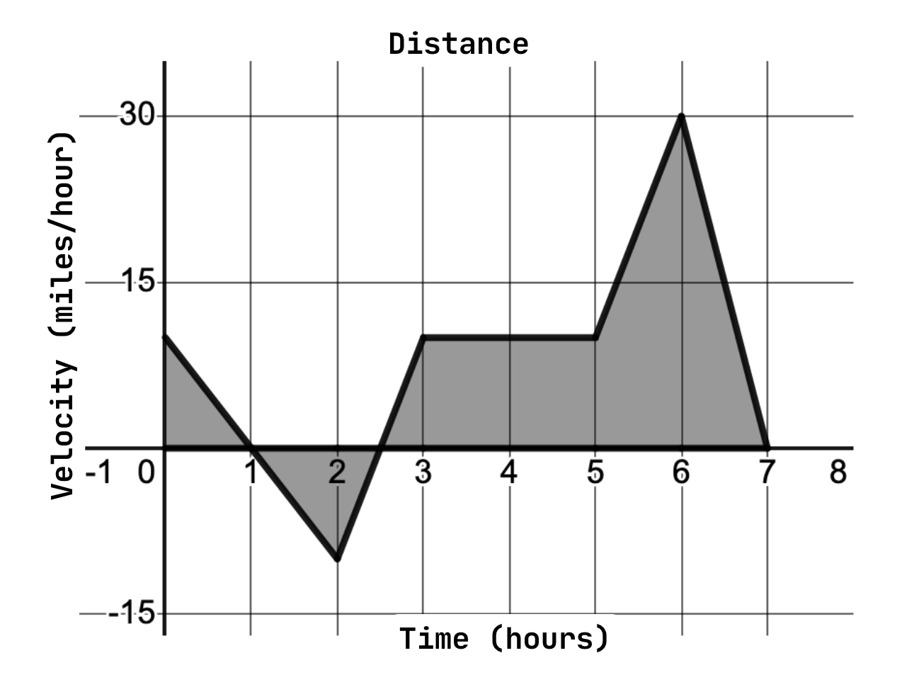
Image courtesy of Emery
Solution: Since this graph is composed entirely of straight lines, we can find the area of each composite shape geometrically. First, let’s draw the shapes we want to find the area of.
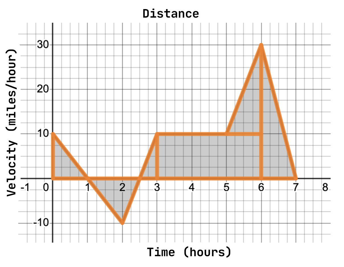
Image courtesy of Emery
We can see that the first triangle has a base of 1 and a height of 10. Using the formula for the area of a triangle, , we find the area to be equal to 5 units. Our next triangle has a base of 1.5 and a height of -10. Applying the same formula, we find its area to be equal to -7.5 units. Importantly, this area is signed, meaning it is negative! In our example scenario, this would be like the car traveling in the opposite direction of its destination.
Our next triangle has a base of 0.5 and a height of 10, for an area of 2.5 units. The large rectangle has a base of 3 and a height of 10, so applying the formula for the area of a rectangle, , we find its area to be equal to 30 units. The triangle sitting on top of it has a base of 1 and a height of 20, for an area of 10 units. Finally, the last triangle has a base of 1 and a height of 30, for an area of 15. Summing these areas, we find the total area under the curve to be:
We learned earlier that our units are the rate of change multiplied by the independent (x-axis) variable, so in this case, we multiply miles/hour by hours. This gives us a unit of miles. Therefore, our car traveled a total of 55 miles toward its destination.
➗ Practice Problems and Solutions
❓Problems
Problem 1: A 50-gallon bathtub is being filled at a constant rate of 10 gal/minute. How long until the bathtub is full?
Problem 2: What is the total, exact area under the curve of the following graph, computed geometrically?
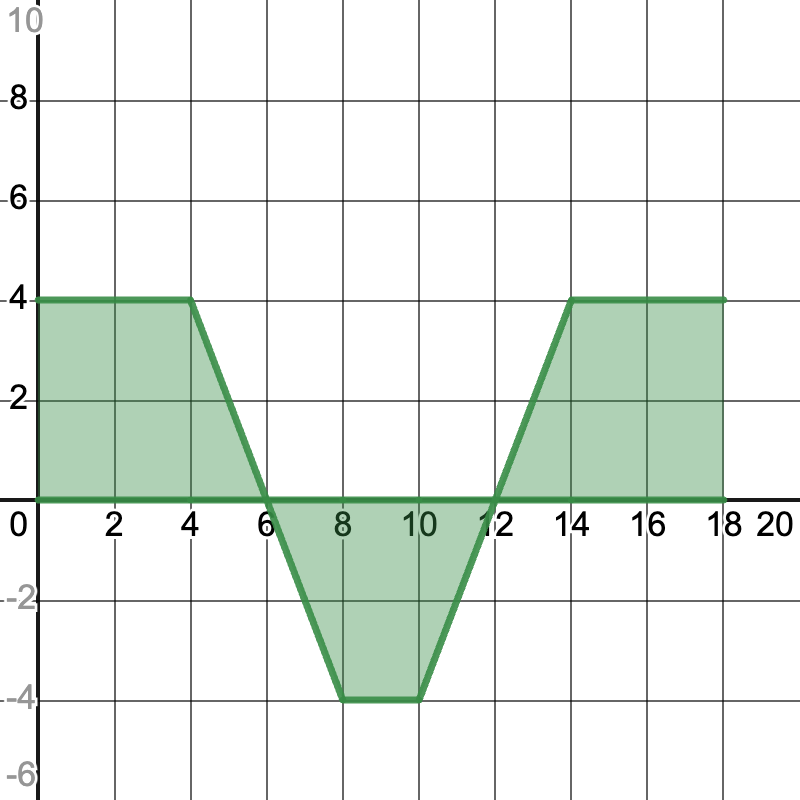
Image courtesy of Emery
Problem 3: What is the area beneath the curve estimated with a Riemann sum of the function using 5 rectangles?
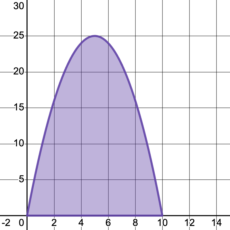
Image courtesy of Emery
💡 Solutions
Problem 1: In this problem, we are given the rate of change, and the end accumulation. We’re missing the “overtime” component. In our very first problem, we found our total accumulation by multiplying the rate of change by our time. So, we used an equation like this: , where is accumulation, is the rate of change, and is time. We can solve for like so: . Applying this to our problem we find that .
Problem 2: Our graph is comprised of three trapezoids. The formula for the area of a trapezoid is
Where and are the two base lengths and is the height. The trapezoids on the right and left side of the graph are identical, with a height of 4 and base heights of 4 and 6. This means they have an area of 20 units. The trapezoid below the x-axis has a height of -4 and base lengths of 2 and 4. Applying our formula, we find it has a signed area of -12. Summing all of these areas, we find the total area under the curve to be 28 .
Problem 3: We first need to draw our rectangles:
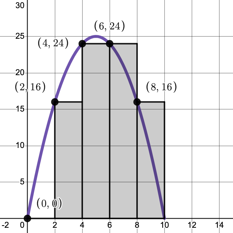
Image courtesy of Emery
Since our graph goes from 0 to 10 and we have five rectangles, we know that each will have a base length of 2. We can use the y-values for each rectangle to get their heights. Thus, we calculate the area to be:
⭐ Closing
After completing this guide, you should be familiar with accumulation of change and how it is represented graphically. You should also feel comfortable applying some basic strategies for calculating accumulation of change over time, and should now be ready to learn more about Riemann sums and integrals!
<< Hide Menu
6.1 Integration and Accumulation of Change
4 min read•june 18, 2024
Emery
Emery
Untitled
Onto unit 6 of AP Calculus! If you were asked to calculate how many miles a car traveled in 3 hours moving at a constant speed of 65 miles per hour, how would you do it? Using this example, you’ll learn about Riemann sums, the basics of integral calculus, and how to apply it to real life!
🏎️ Change Over Time
Accumulation of change is exactly what it sounds like—the sum, over time, of how much something has changed. Let’s return to the example at the beginning: we want to know how far a car has traveled, and we are given its speed (in miles per hour) and the length of time it has been traveling. We want to know how many miles it has accumulated over 3 hours. This problem is fairly straightforward, and we can solve it with a simple equation:
where d is distance, v is velocity (speed), and t is time. Let’s apply it to the problem.
Notice that because we have the unit hours in the denominator of one term and the numerator of the other, they cancel, leaving us with just a unit of miles. This is how units will work for all of these problems—they should be the unit of the rate of change multiplied by the independent variable.
We’ve solved our first problem! Now, let’s connect it to calculus.
📈 Graphing Change Over Time
We can depict the relationship between how fast, how long, and how far the car traveled with a graph.

Image courtesy of Emery
Here, we can see that the x-axis represents how long the car has been traveling and the y-axis represents how fast it is traveling. The shaded area under the curve represents the total distance traveled.
This example is about a car that is traveling at a constant speed, as though it was on the highway using cruise control. But in reality, a whole trip for a vehicle involves variation in speed. Let’s look at another example, where a car leaves its house, accelerates to 50 miles per hours, drives on the highway for almost two hours, decelerates to 20 miles per hour, finishes driving to its destination, and then decelerates to 0 miles per hour. How far did the car travel?

Image courtesy of Emery
Based on our simpler example, we know that the shaded area under the curve will give us the distance the car traveled. But, we can’t just use the equation for an area of a rectangle here, because it’s a much more complex shape! The following piecewise function describes the curve:
There are a few different ways we can approach this problem: by estimating using rectangles, or by using an integral.
📊 Riemann Sums
The first way we can find area under the curve is by using something called a Riemann Sum. This involves drawing rectangles, or other easy shapes to take the area of, and using them to approximate the area under the curve. Let’s apply it to our problem!
✏️ Riemann Sum: Step-by-Step
Step 1: How Many Rectangles?
The first thing we need to do is decide how many rectangles we want to use to approximate our area under the curve. For simplicity’s sake, let’s just use six in this example. We want them to have equal widths, so we divide our total base by our number of rectangles. Since the car’s trip was three hours long, we’ll divide 3 by 6, to find a base length of 0.5. Step 2: Graphing****
Let’s add our six rectangles to our initial graph:

Image courtesy of Emery
Step 3: Computation
Finally, let’s create a table and calculate the area of each rectangle. Our table of values looks like this:
| Base | Height |
| 0.5 | 0 |
| 0.5 | 50 |
| 0.5 | 50 |
| 0.5 | 50 |
| 0.5 | 50 |
| 0.5 | 20 |
To calculate the total area, we will sum the areas of each of these rectangles like so:
Since our base length is the same, we can factor it out and simplify our equation like this:
Therefore, using this simple approximation, we find that our car has traveled about 110 miles! However, based on the graph, we can see that this is probably somewhat inaccurate, as it includes both overestimations and underestimations of the true distance traveled. This is where integrals come in!
📈 Preview of Integrals
So far, we’ve worked on approximating the area under the curve, or the accumulation of change. But, we have a very powerful tool at our disposal—the integral. Integrals are also called anti-derivatives, which is exactly what it sounds like! They “undo” derivation, just like multiplication undoes division. They also calculate the exact area under the curve.
Integration is represented with the following notation:
This notation tells us to find the area under the curve for our function over the interval [0,3]. This type of integral is specifically called a definite integral. We won’t cover how to take the integral right now, but if you did take it, you would find that the exact area under the curve in our example problem is 117.44 miles.
📝 Practice
Let’s look at one final sample problem before trying it on your own!
Example Problem: Consider the following graph of the function , which represents the total distance traveled by a vehicle over time. What is the average speed of the vehicle?

Image courtesy of Emery
Solution: Since this graph is composed entirely of straight lines, we can find the area of each composite shape geometrically. First, let’s draw the shapes we want to find the area of.

Image courtesy of Emery
We can see that the first triangle has a base of 1 and a height of 10. Using the formula for the area of a triangle, , we find the area to be equal to 5 units. Our next triangle has a base of 1.5 and a height of -10. Applying the same formula, we find its area to be equal to -7.5 units. Importantly, this area is signed, meaning it is negative! In our example scenario, this would be like the car traveling in the opposite direction of its destination.
Our next triangle has a base of 0.5 and a height of 10, for an area of 2.5 units. The large rectangle has a base of 3 and a height of 10, so applying the formula for the area of a rectangle, , we find its area to be equal to 30 units. The triangle sitting on top of it has a base of 1 and a height of 20, for an area of 10 units. Finally, the last triangle has a base of 1 and a height of 30, for an area of 15. Summing these areas, we find the total area under the curve to be:
We learned earlier that our units are the rate of change multiplied by the independent (x-axis) variable, so in this case, we multiply miles/hour by hours. This gives us a unit of miles. Therefore, our car traveled a total of 55 miles toward its destination.
➗ Practice Problems and Solutions
❓Problems
Problem 1: A 50-gallon bathtub is being filled at a constant rate of 10 gal/minute. How long until the bathtub is full?
Problem 2: What is the total, exact area under the curve of the following graph, computed geometrically?

Image courtesy of Emery
Problem 3: What is the area beneath the curve estimated with a Riemann sum of the function using 5 rectangles?

Image courtesy of Emery
💡 Solutions
Problem 1: In this problem, we are given the rate of change, and the end accumulation. We’re missing the “overtime” component. In our very first problem, we found our total accumulation by multiplying the rate of change by our time. So, we used an equation like this: , where is accumulation, is the rate of change, and is time. We can solve for like so: . Applying this to our problem we find that .
Problem 2: Our graph is comprised of three trapezoids. The formula for the area of a trapezoid is
Where and are the two base lengths and is the height. The trapezoids on the right and left side of the graph are identical, with a height of 4 and base heights of 4 and 6. This means they have an area of 20 units. The trapezoid below the x-axis has a height of -4 and base lengths of 2 and 4. Applying our formula, we find it has a signed area of -12. Summing all of these areas, we find the total area under the curve to be 28 .
Problem 3: We first need to draw our rectangles:

Image courtesy of Emery
Since our graph goes from 0 to 10 and we have five rectangles, we know that each will have a base length of 2. We can use the y-values for each rectangle to get their heights. Thus, we calculate the area to be:
⭐ Closing
After completing this guide, you should be familiar with accumulation of change and how it is represented graphically. You should also feel comfortable applying some basic strategies for calculating accumulation of change over time, and should now be ready to learn more about Riemann sums and integrals!

© 2025 Fiveable Inc. All rights reserved.