Jeanne Stansak
dylan_black_2025
Jeanne Stansak
dylan_black_2025
What is Production?
So far in microeconomics, we've defined consumers and producers as our two main subjects. We've done quite a bit so far in our study of consumer theory. Consumer theory attempts to understand how consumers act and maximize their utility, which we did some of in units 1 and 2. In unit 3, and for much of the rest of AP Micro, we'll turn to producers and aim to understand how producers act under different market structures.
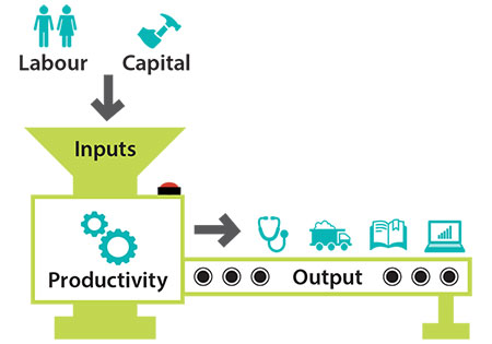
The first step to understanding producers, also known as the theory of the firm, is to understand what exactly production is. This may sound simple, but it's worth getting a strict definition. In economics, production refers to the process by which a producer takes inputs, or factors of production, and creates an output. An input is defined as any resource used by a firm to create an output. The common factors of production are land, labor, and capital, but it also varies. For example, a pizza parlor uses tomatoes, yeast, and flour. These are inputs to the creation of an output, pizza.

Costs of Production and Revenue
When a firm produces goods, there are also costs associated with those goods. There are two primary types of costs: fixed costs, which are costs that don't scale with output, and variable costs, costs that do scale with output. For example, a business needs to pay for their rent each month, but this does not scale up or down based on the amount of pizza produced. However, the cost of tomatoes does scale, since the more pizzas we make, the more we pay for tomatoes. We'll elaborate on these costs in the next section.
When a firm sells a good, they receive revenue. Revenue is the total amount of money a firm brings in. Total revenue is calculated with the formula TR = P*Q, since if we sell Q units at price P, we make PQ. After accounting for the costs, we're left with profit. These are two kinds of profit: accounting profit and economic profit. Accounting profit is the profit you're most familiar with: it's simply the amount of money a business makes. Economic profit, on the other hand, takes into account opportunity cost. This becomes clearer with an example.
Suppose Michael Jordan has two choices: open a pizza shop and earn 1,000,000. If he opens the pizza shop, his accounting profit would be 1,000,000 he could have earned in the NBA, so his economic profit is actually -$950,000.

You on your AP Micro exams...unfortunately you don't get paid $1,000,000 to take those
Measuring Productivity
We have a few ways of measuring how much a firm produces. The first is simply total product (TP), in which we measure how much a firm output. This is the most clear and simple way of viewing productivity: with some inputs, we produce some total product. However, this may not tell the whole story.
We can also look at average product (AP) by dividing total product by the number of inputs. For example, if we produce a total of 50 units with 2 workers, our average product is 25 units.
Finally, we can calculate marginal product (MP). Marginal product is the additional output from adding one more input. For example, if we produce 50 units with 2 workers and 60 with 3, our marginal product from the third worker was 10 units. Marginal product is especially useful because it helps us measure how many inputs we should use. If marginal product ever reaches zero or negatives, we should not add that additional output.
The Law of Diminishing Marginal Product
The Law of Diminishing Marginal product is a property of marginal product that states that as we add more inputs, the additional product we receive from each input diminishes. Eventually, our marginal product will always reach zero and then enter the negatives. For a time, we may see increasing marginal product, in which MP is increasing, but eventually, we will reach a point of diminishing marginal returns. Eventually, we'll always reach negative marginal returns.
For example, suppose a pizza shop is hiring workers. With 1 worker, we may produce 10 pizzas, so MP = 10. Then, if we hire a second worker, we may produce 25 pizzas, so we have an MP = 15, meaning we've experienced increasing marginal returns. However, let's say the third worker only brings us up to 30 pizzas. We've still increased production, but only with a marginal product of 5. We've experienced diminishing marginal returns. Let's suppose that our fourth worker keeps bumping into people and actually keeps us at production of 30 pizzas. Their marginal product is zero. Finally, we hire a fifth worker. Let's suppose that at this point, our work space is so crowded that we make 25 pizzas. This means the marginal product of the fifth worker was actually negative 5 pizzas.
The following table and graph may give a better picture:


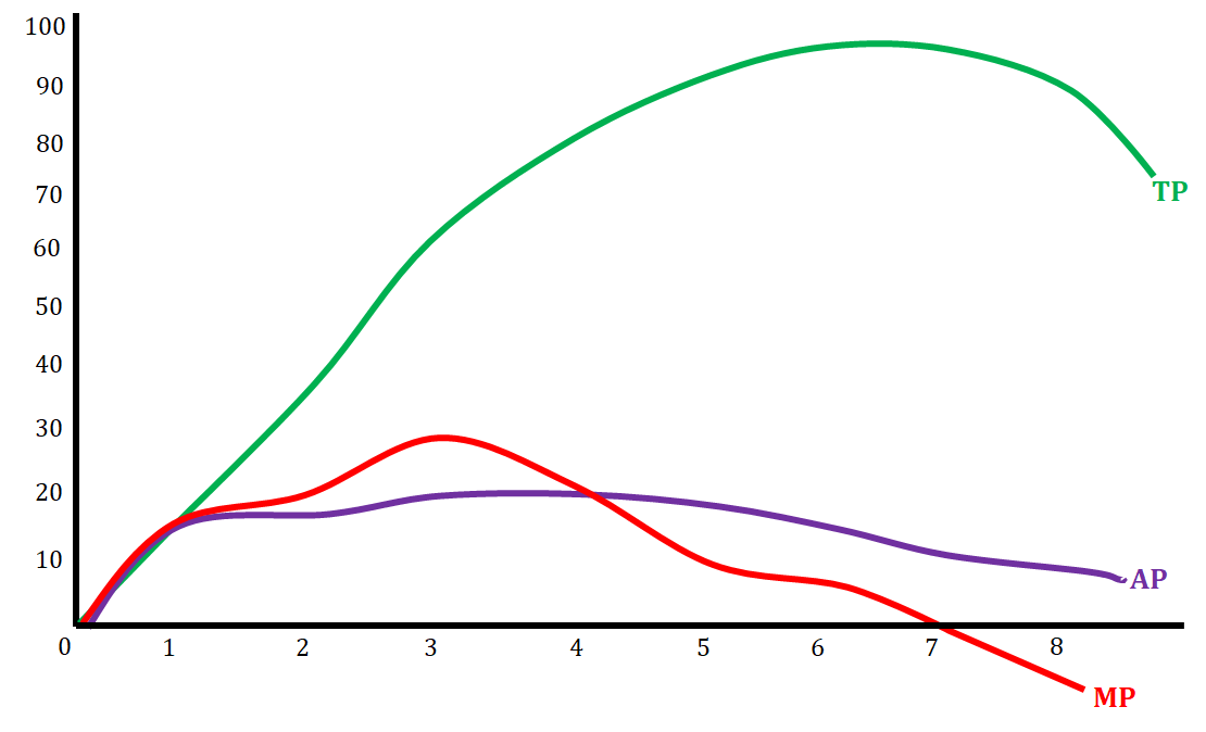
The above graph shows how total product, average product, and marginal product are related when placed on a graph. There are some basic facts about how these particular curves are related:
- When marginal product is increasing, total product is increasing at an increasing rate. The slope is steeper.
- When marginal product is decreasing, total product is increasing at a decreasing (slower) rate. The slope is less steep.
- When marginal product becomes negative, total product is decreasing.
Returns to Scale
Finally, we can understand how our output scales with our inputs. Returns to scale refers to the idea that as we scale our inputs, production should scale proportionally. With increasing returns to scale, we see production more than double when we double inputs. Decreasing returns to scale are the opposite, with production less than doubling when we double inputs. Finally, returns to scale implies that doubling inputs will perfectly double output.

<< Hide Menu
Jeanne Stansak
dylan_black_2025
Jeanne Stansak
dylan_black_2025
What is Production?
So far in microeconomics, we've defined consumers and producers as our two main subjects. We've done quite a bit so far in our study of consumer theory. Consumer theory attempts to understand how consumers act and maximize their utility, which we did some of in units 1 and 2. In unit 3, and for much of the rest of AP Micro, we'll turn to producers and aim to understand how producers act under different market structures.
The first step to understanding producers, also known as the theory of the firm, is to understand what exactly production is. This may sound simple, but it's worth getting a strict definition. In economics, production refers to the process by which a producer takes inputs, or factors of production, and creates an output. An input is defined as any resource used by a firm to create an output. The common factors of production are land, labor, and capital, but it also varies. For example, a pizza parlor uses tomatoes, yeast, and flour. These are inputs to the creation of an output, pizza.

Costs of Production and Revenue
When a firm produces goods, there are also costs associated with those goods. There are two primary types of costs: fixed costs, which are costs that don't scale with output, and variable costs, costs that do scale with output. For example, a business needs to pay for their rent each month, but this does not scale up or down based on the amount of pizza produced. However, the cost of tomatoes does scale, since the more pizzas we make, the more we pay for tomatoes. We'll elaborate on these costs in the next section.
When a firm sells a good, they receive revenue. Revenue is the total amount of money a firm brings in. Total revenue is calculated with the formula TR = P*Q, since if we sell Q units at price P, we make PQ. After accounting for the costs, we're left with profit. These are two kinds of profit: accounting profit and economic profit. Accounting profit is the profit you're most familiar with: it's simply the amount of money a business makes. Economic profit, on the other hand, takes into account opportunity cost. This becomes clearer with an example.
Suppose Michael Jordan has two choices: open a pizza shop and earn 1,000,000. If he opens the pizza shop, his accounting profit would be 1,000,000 he could have earned in the NBA, so his economic profit is actually -$950,000.

You on your AP Micro exams...unfortunately you don't get paid $1,000,000 to take those
Measuring Productivity
We have a few ways of measuring how much a firm produces. The first is simply total product (TP), in which we measure how much a firm output. This is the most clear and simple way of viewing productivity: with some inputs, we produce some total product. However, this may not tell the whole story.
We can also look at average product (AP) by dividing total product by the number of inputs. For example, if we produce a total of 50 units with 2 workers, our average product is 25 units.
Finally, we can calculate marginal product (MP). Marginal product is the additional output from adding one more input. For example, if we produce 50 units with 2 workers and 60 with 3, our marginal product from the third worker was 10 units. Marginal product is especially useful because it helps us measure how many inputs we should use. If marginal product ever reaches zero or negatives, we should not add that additional output.
The Law of Diminishing Marginal Product
The Law of Diminishing Marginal product is a property of marginal product that states that as we add more inputs, the additional product we receive from each input diminishes. Eventually, our marginal product will always reach zero and then enter the negatives. For a time, we may see increasing marginal product, in which MP is increasing, but eventually, we will reach a point of diminishing marginal returns. Eventually, we'll always reach negative marginal returns.
For example, suppose a pizza shop is hiring workers. With 1 worker, we may produce 10 pizzas, so MP = 10. Then, if we hire a second worker, we may produce 25 pizzas, so we have an MP = 15, meaning we've experienced increasing marginal returns. However, let's say the third worker only brings us up to 30 pizzas. We've still increased production, but only with a marginal product of 5. We've experienced diminishing marginal returns. Let's suppose that our fourth worker keeps bumping into people and actually keeps us at production of 30 pizzas. Their marginal product is zero. Finally, we hire a fifth worker. Let's suppose that at this point, our work space is so crowded that we make 25 pizzas. This means the marginal product of the fifth worker was actually negative 5 pizzas.
The following table and graph may give a better picture:


The above graph shows how total product, average product, and marginal product are related when placed on a graph. There are some basic facts about how these particular curves are related:
- When marginal product is increasing, total product is increasing at an increasing rate. The slope is steeper.
- When marginal product is decreasing, total product is increasing at a decreasing (slower) rate. The slope is less steep.
- When marginal product becomes negative, total product is decreasing.
Returns to Scale
Finally, we can understand how our output scales with our inputs. Returns to scale refers to the idea that as we scale our inputs, production should scale proportionally. With increasing returns to scale, we see production more than double when we double inputs. Decreasing returns to scale are the opposite, with production less than doubling when we double inputs. Finally, returns to scale implies that doubling inputs will perfectly double output.


© 2024 Fiveable Inc. All rights reserved.