Browse By Unit
1.3 Rates of Change in Linear and Quadratic Functions
1 min read•june 18, 2024
1.3 Rates of Change in Linear and Quadratic Functions
📈 Average Rates of Change
A linear function is one in which the output value changes proportionally with the input value, resulting in a straight line when graphed. ✏️
The average rate of change over any interval of the input values is constant because the slope, or rate of change, of the line remains constant throughout.
A quadratic function, on the other hand, involves a squared term in the input value, resulting in a curved graph.
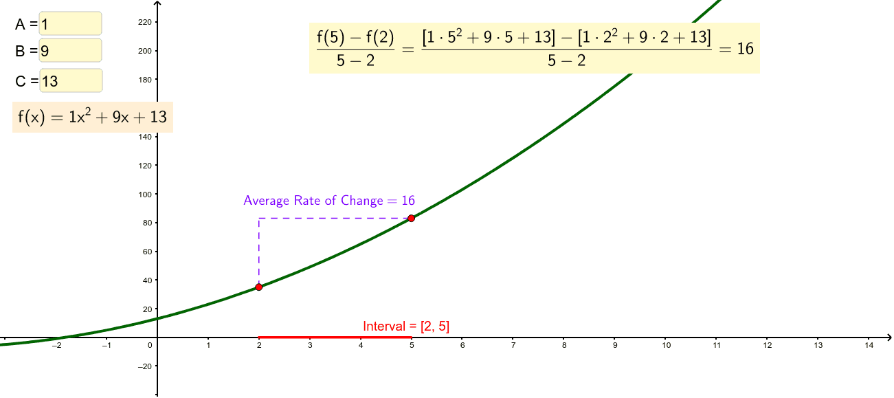
The average rate of change over consecutive equal-length intervals of the input values can be calculated and represented by a linear function, as the slope of the curve changes continuously. This linear function is the tangent line to the curve at the midpoint of each interval and approximates the rate of change of the function over that interval.

Image Courtesy of Geogebra
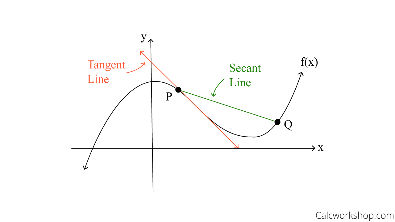
The average rate of change can be visualized by drawing a line connecting two points on the function, namely, (a, f(a)) and (b, f(b)). This line is known as the secant line, and the slope of this line represents the average rate of change of the function over the interval [a, b]. In other words, the slope of the secant line indicates how much the output value of the function changes for every unit increase in the input value over the interval [a, b]! 🙈

Image Courtesy of Calc Workshop
📐 Change in Average Rates of Change
A linear function is characterized by a constant rate of change over its entire domain. Thus, the average rate of change of a linear function over any consecutive equal-length input-value intervals is also a constant function. As a result, the average rates of change for a linear function do not change over the course of the function.
In other words, the function is not accelerating or decelerating; the rates of change remain constant. 🚗
For a quadratic function, the rate of change is not constant. Instead, it varies continuously throughout the function. However, the average rates of change over consecutive equal-length input-value intervals can be approximated by a linear function.
Therefore, the rate of change for a quadratic function is changing at a constant rate, but the rate of change itself is not constant. This means that the function is accelerating or decelerating at a constant rate, depending on the sign of the leading coefficient of the quadratic term.
📝 A Note on Concavity
When the average rate of change over equal-length input-value intervals is increasing for all small-length intervals, it implies that the function is increasing at an increasing rate, which means that the graph of the function is curving upwards or concave up. ⤴️
On the other hand, when the average rate of change over equal-length input-value intervals is decreasing for all small-length intervals, it implies that the function is decreasing at an increasing rate, which means that the graph of the function is curving downwards or concave down. ⤵️
Altogether, the concavity of the graph of a function can provide useful information about the behavior of the function, such as the location of its maximum and minimum points.
<< Hide Menu
1.3 Rates of Change in Linear and Quadratic Functions
1 min read•june 18, 2024
1.3 Rates of Change in Linear and Quadratic Functions
📈 Average Rates of Change
A linear function is one in which the output value changes proportionally with the input value, resulting in a straight line when graphed. ✏️
The average rate of change over any interval of the input values is constant because the slope, or rate of change, of the line remains constant throughout.
A quadratic function, on the other hand, involves a squared term in the input value, resulting in a curved graph.
The average rate of change over consecutive equal-length intervals of the input values can be calculated and represented by a linear function, as the slope of the curve changes continuously. This linear function is the tangent line to the curve at the midpoint of each interval and approximates the rate of change of the function over that interval.

Image Courtesy of Geogebra
The average rate of change can be visualized by drawing a line connecting two points on the function, namely, (a, f(a)) and (b, f(b)). This line is known as the secant line, and the slope of this line represents the average rate of change of the function over the interval [a, b]. In other words, the slope of the secant line indicates how much the output value of the function changes for every unit increase in the input value over the interval [a, b]! 🙈

Image Courtesy of Calc Workshop
📐 Change in Average Rates of Change
A linear function is characterized by a constant rate of change over its entire domain. Thus, the average rate of change of a linear function over any consecutive equal-length input-value intervals is also a constant function. As a result, the average rates of change for a linear function do not change over the course of the function.
In other words, the function is not accelerating or decelerating; the rates of change remain constant. 🚗
For a quadratic function, the rate of change is not constant. Instead, it varies continuously throughout the function. However, the average rates of change over consecutive equal-length input-value intervals can be approximated by a linear function.
Therefore, the rate of change for a quadratic function is changing at a constant rate, but the rate of change itself is not constant. This means that the function is accelerating or decelerating at a constant rate, depending on the sign of the leading coefficient of the quadratic term.
📝 A Note on Concavity
When the average rate of change over equal-length input-value intervals is increasing for all small-length intervals, it implies that the function is increasing at an increasing rate, which means that the graph of the function is curving upwards or concave up. ⤴️
On the other hand, when the average rate of change over equal-length input-value intervals is decreasing for all small-length intervals, it implies that the function is decreasing at an increasing rate, which means that the graph of the function is curving downwards or concave down. ⤵️
Altogether, the concavity of the graph of a function can provide useful information about the behavior of the function, such as the location of its maximum and minimum points.

© 2024 Fiveable Inc. All rights reserved.