Browse By Unit
Jesse
Jesse
4.13 Matrices as Functions
Connecting Linear Transformations and Matrices
The linear transformation mapping a vector to a vector can be represented by a matrix [a₁₁ a₁₂; a₂₁ a₂₂] (a clearer image shown below), known as a 2 x 2 matrix. This matrix is called a transformation matrix, and it encodes all the information about the linear transformation, including the coefficients a₁₁, a₁₂, a₂₁, and a₂₂. 📜
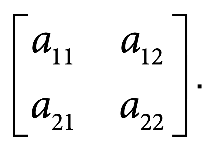
Image Created by Jed Q
When the vector is multiplied by the matrix [a₁₁ a₁₂; a₂₁ a₂₂], it results in a new vector , which is the image of the original vector under the linear transformation. 🔦
This idea can be extended to n-dimensional space, where a linear transformation mapping a vector to a vector can be represented by an n x n matrix, where each element aij is the coefficient for the xj component of the output vector.
The mapping of the unit vectors in a linear transformation can provide valuable information for determining the associated matrix. In a two-dimensional space, the unit vectors are the vectors and . These vectors are often referred to as the "standard basis" vectors. The linear transformation maps these unit vectors to new vectors in the transformed space. The components of these new vectors are the columns of the transformation matrix. 🗺️
For example, if the linear transformation maps the unit vector to the vector and the unit vector to the vector , the transformation matrix is [a₁₁ a₁₂; a₂₁ a₂₂].
In higher dimensional spaces, the unit vectors are the vectors with a single component equal to 1 1️⃣ and all other components equal to 0. 0️⃣ The linear transformation maps these unit vectors to new vectors in the transformed space. The components of these new vectors are the columns of the transformation matrix. 🔢
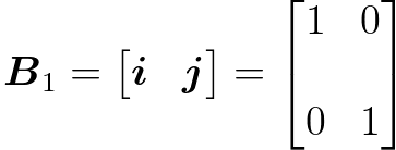
Image Courtesy of Towards Data Science
Involving Angles
The matrix associated with a linear transformation of vectors that maps every vector to the vector that is an angle θ counterclockwise rotation about the origin from the original vector is (see image below). This is known as the rotation matrix. 🌀
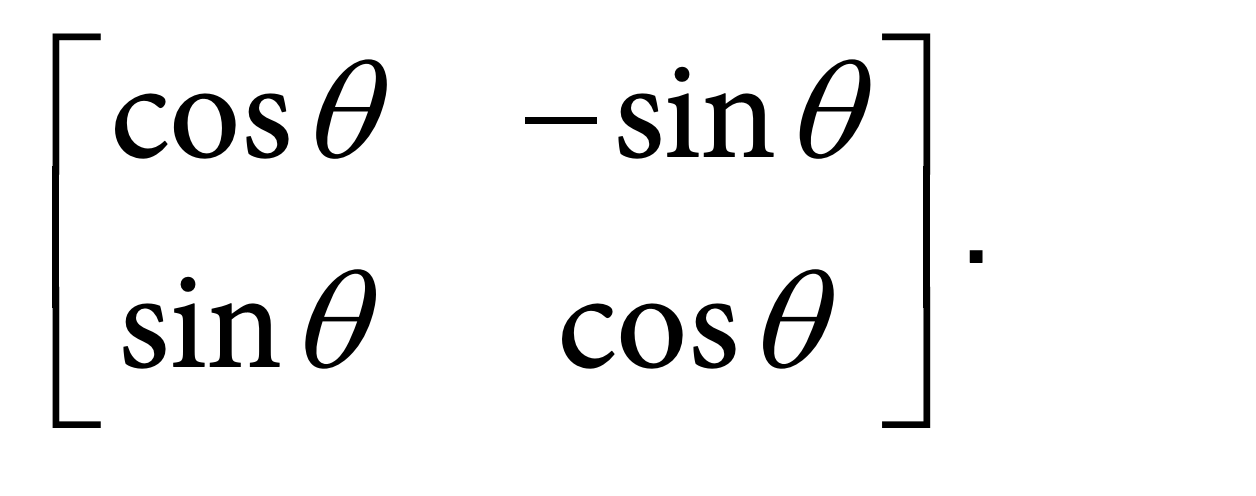
Image Created by Jed Q
When a vector is multiplied by this matrix, the resulting vector is the image of the original vector under the rotation transformation. The transformation can be described as:
This means that x' and y' are the coordinates of the vector after it has been rotated by an angle θ counterclockwise. The matrix [cosθ −sinθ; sinθ cosθ] encodes all the information about the rotation transformation, including the angle of rotation θ. 📐
It is also important to note that the matrix [cos(−θ) −sin(−θ); sin(−θ) cos(−θ)] will give the same transformation but clockwise rotation. ⏰

Image Courtesy of Math Stack Exchange
Absolute Values & Determinants
The absolute value of the determinant of a 2 x 2 transformation matrix gives the magnitude of the dilation of regions in R2 under the transformation. The determinant of a matrix is a scalar value that can be calculated from the elements of a matrix. The determinant of a 2x2 matrix is given by the formula . ⏸
In the case of a linear transformation, the determinant represents the scaling factor of the transformation.
- A positive determinant indicates that the transformation is a dilation, meaning that it increases the size of a region. ➕
- A negative determinant indicates a reflection, meaning that it changes the orientation of the region. ➖
For example, if the determinant of a 2x2 matrix is 2, it means that the transformation associated with that matrix is a dilation that increases the size of a region by a factor of 2. Similarly, if the determinant is -3, it means that the transformation is a dilation that decreases the size of a region by a factor of 3 and also changes the orientation of the region. ✂️
Compositions of Two Linear Transformations
The composition of two linear transformations is a linear transformation. Remember, a linear transformation is a function that takes a vector as an input and produces another vector as an output. When two linear transformations are composed, the output of the first transformation is used as the input for the second transformation. 👗
For example, if f(x) is a linear transformation that maps a vector x to a vector y and g(x) is another linear transformation that maps a vector y to a vector z, the composition of f and g is denoted as g(f(x)) and it maps the vector x to the vector z.
The composition of two linear transformations is associative, meaning that , the order of the linear transformations does not affect the result. 🙅
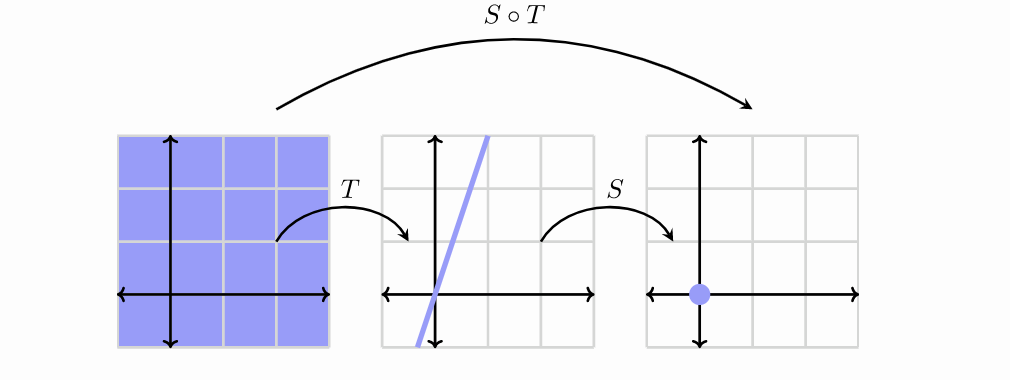
Image Courtesy of Ximera (Ohio State University)
The matrix associated with the composition of two linear transformations is the product of the matrices associated with each linear transformation. For example, if A is the matrix associated with the linear transformation f and B is the matrix associated with the linear transformation g, the matrix associated with the composition of f and g is AB. ⚡️
When a vector x is multiplied by the matrix AB, it results in a new vector y, which is the image of the original vector under the composition of the linear transformations f and g.
Inverses of Linear Transformations
Two linear transformations are said to be inverses if their composition maps any vector to itself. An inverse transformation is a transformation that "undoes" the effect of another transformation. In other words, if a linear transformation "f" maps a vector "x" to a vector "y" and another linear transformation "g" maps the vector "y" back to the vector "x", the transformation "g" is said to be the inverse of the transformation "f" and is denoted as "f^-1" 🔃
Formally, if f: V → W and g: W → V are linear transformations, they are inverses if and only if for all x in V and for all y in W.
The composition of two linear transformations is commutative, meaning that f(g(x)) = g(f(x)), so either order of the linear transformations will result in the same outcome, the identity transformation. 🙋
If a linear transformation, L, is given by , where A is a matrix and v is a vector, then its inverse transformation, denoted as L^-1, is given by , where A^-1 is the inverse of the matrix A.
This relationship between the linear transformation L, its matrix representation A, and its inverse transformation L^-1, is a direct consequence of the properties of matrix-vector multiplication. The matrix A encodes the linear transformation L, and the vector v is transformed by A to produce the output vector Av. 🤝
The inverse of a matrix A is a matrix A^-1 such that when it's multiplied by A, the result is the identity matrix I. This means that . It's important to note that not every matrix has an inverse. A matrix A is invertible if and only if its determinant is non-zero.
By applying the inverse matrix A^-1 to the output vector Av, we obtain the original vector v. This is the inverse transformation L^-1. In other words, . 🤓

Image Courtesy of Ximera (Ohio State University)
<< Hide Menu
Jesse
Jesse
4.13 Matrices as Functions
Connecting Linear Transformations and Matrices
The linear transformation mapping a vector to a vector can be represented by a matrix [a₁₁ a₁₂; a₂₁ a₂₂] (a clearer image shown below), known as a 2 x 2 matrix. This matrix is called a transformation matrix, and it encodes all the information about the linear transformation, including the coefficients a₁₁, a₁₂, a₂₁, and a₂₂. 📜

Image Created by Jed Q
When the vector is multiplied by the matrix [a₁₁ a₁₂; a₂₁ a₂₂], it results in a new vector , which is the image of the original vector under the linear transformation. 🔦
This idea can be extended to n-dimensional space, where a linear transformation mapping a vector to a vector can be represented by an n x n matrix, where each element aij is the coefficient for the xj component of the output vector.
The mapping of the unit vectors in a linear transformation can provide valuable information for determining the associated matrix. In a two-dimensional space, the unit vectors are the vectors and . These vectors are often referred to as the "standard basis" vectors. The linear transformation maps these unit vectors to new vectors in the transformed space. The components of these new vectors are the columns of the transformation matrix. 🗺️
For example, if the linear transformation maps the unit vector to the vector and the unit vector to the vector , the transformation matrix is [a₁₁ a₁₂; a₂₁ a₂₂].
In higher dimensional spaces, the unit vectors are the vectors with a single component equal to 1 1️⃣ and all other components equal to 0. 0️⃣ The linear transformation maps these unit vectors to new vectors in the transformed space. The components of these new vectors are the columns of the transformation matrix. 🔢

Image Courtesy of Towards Data Science
Involving Angles
The matrix associated with a linear transformation of vectors that maps every vector to the vector that is an angle θ counterclockwise rotation about the origin from the original vector is (see image below). This is known as the rotation matrix. 🌀

Image Created by Jed Q
When a vector is multiplied by this matrix, the resulting vector is the image of the original vector under the rotation transformation. The transformation can be described as:
This means that x' and y' are the coordinates of the vector after it has been rotated by an angle θ counterclockwise. The matrix [cosθ −sinθ; sinθ cosθ] encodes all the information about the rotation transformation, including the angle of rotation θ. 📐
It is also important to note that the matrix [cos(−θ) −sin(−θ); sin(−θ) cos(−θ)] will give the same transformation but clockwise rotation. ⏰

Image Courtesy of Math Stack Exchange
Absolute Values & Determinants
The absolute value of the determinant of a 2 x 2 transformation matrix gives the magnitude of the dilation of regions in R2 under the transformation. The determinant of a matrix is a scalar value that can be calculated from the elements of a matrix. The determinant of a 2x2 matrix is given by the formula . ⏸
In the case of a linear transformation, the determinant represents the scaling factor of the transformation.
- A positive determinant indicates that the transformation is a dilation, meaning that it increases the size of a region. ➕
- A negative determinant indicates a reflection, meaning that it changes the orientation of the region. ➖
For example, if the determinant of a 2x2 matrix is 2, it means that the transformation associated with that matrix is a dilation that increases the size of a region by a factor of 2. Similarly, if the determinant is -3, it means that the transformation is a dilation that decreases the size of a region by a factor of 3 and also changes the orientation of the region. ✂️
Compositions of Two Linear Transformations
The composition of two linear transformations is a linear transformation. Remember, a linear transformation is a function that takes a vector as an input and produces another vector as an output. When two linear transformations are composed, the output of the first transformation is used as the input for the second transformation. 👗
For example, if f(x) is a linear transformation that maps a vector x to a vector y and g(x) is another linear transformation that maps a vector y to a vector z, the composition of f and g is denoted as g(f(x)) and it maps the vector x to the vector z.
The composition of two linear transformations is associative, meaning that , the order of the linear transformations does not affect the result. 🙅

Image Courtesy of Ximera (Ohio State University)
The matrix associated with the composition of two linear transformations is the product of the matrices associated with each linear transformation. For example, if A is the matrix associated with the linear transformation f and B is the matrix associated with the linear transformation g, the matrix associated with the composition of f and g is AB. ⚡️
When a vector x is multiplied by the matrix AB, it results in a new vector y, which is the image of the original vector under the composition of the linear transformations f and g.
Inverses of Linear Transformations
Two linear transformations are said to be inverses if their composition maps any vector to itself. An inverse transformation is a transformation that "undoes" the effect of another transformation. In other words, if a linear transformation "f" maps a vector "x" to a vector "y" and another linear transformation "g" maps the vector "y" back to the vector "x", the transformation "g" is said to be the inverse of the transformation "f" and is denoted as "f^-1" 🔃
Formally, if f: V → W and g: W → V are linear transformations, they are inverses if and only if for all x in V and for all y in W.
The composition of two linear transformations is commutative, meaning that f(g(x)) = g(f(x)), so either order of the linear transformations will result in the same outcome, the identity transformation. 🙋
If a linear transformation, L, is given by , where A is a matrix and v is a vector, then its inverse transformation, denoted as L^-1, is given by , where A^-1 is the inverse of the matrix A.
This relationship between the linear transformation L, its matrix representation A, and its inverse transformation L^-1, is a direct consequence of the properties of matrix-vector multiplication. The matrix A encodes the linear transformation L, and the vector v is transformed by A to produce the output vector Av. 🤝
The inverse of a matrix A is a matrix A^-1 such that when it's multiplied by A, the result is the identity matrix I. This means that . It's important to note that not every matrix has an inverse. A matrix A is invertible if and only if its determinant is non-zero.
By applying the inverse matrix A^-1 to the output vector Av, we obtain the original vector v. This is the inverse transformation L^-1. In other words, . 🤓

Image Courtesy of Ximera (Ohio State University)

© 2024 Fiveable Inc. All rights reserved.