Browse By Unit
Dalia Savy
Jacob Jeffries
Dalia Savy
Jacob Jeffries
After plenty of math, we're back to the conceptual part of this unit! Remember that kinetics is the study of the rate of chemical reactions, or basically, how fast a chemical reaction can go. In this study guide, you'll learn that in order for a reaction to proceed, or be successful, very specific conditions must be satisfied.
What is the Collision Model?
The collision model essentially models molecules as projectiles moving in random directions with a fixed average speed that is determined by temperature. As these projectiles collide, they bounce off one another, preserving their kinetic energy and momentum. Thus, through this model, one can see that a reaction is nothing more than two atoms or molecules essentially slamming into each other with:
- enough energy to cause a reaction (the energy needed to cause a reaction is called the activation energy), and
- the correct orientation to form products. This can be seen in the following image:

Image Courtesy of SaylorDotOrg
As we can see in this image, two molecules, nitrogen monoxide and ozone, slam together in an effective collision (we'll see what that means a bit later) to form nitrogen dioxide and molecular oxygen. This reaction serves as an example of what occurs during a chemical reaction according to the kinetic collision model.
The Math Behind the Model
⚠️ You do not need to know this section, but it is worth a read-through to better conceptually understand this model.
An important distinction to recognize is that these collisions are not actually random. Two particles colliding with one another have a very well-defined system of equations that one can use to solve for their trajectories. The first one is the statement about the conservation of kinetic energy:
The second one is the statement of conservation of momentum:
- m1 and m2 both describe the masses of particle 1 and particle 2,
- v1,i and v2,i both describe the initial velocities of particle 1 and 2 before the collision,
- and v1,f, and v2,f both define the final velocities of 1 and 2 after the collision. Qualitatively, Eq. 10 states that the total kinetic energy of the system stays constant, and Eq. 11 states that the total momentum of the system also stays constant.
However, a modification must be made to accurately describe reactive collisions (ie. a collision where a chemical reaction happens), as some of the kinetic energy must be expended to break and create new chemical bonds, thus making the system’s total kinetic energy a non-constant variable.
These equations by themselves are not very useful on a macroscopic scale. These collisions take place within systems of many molecules, and Eq. 10 and Eq. 11 only describe two-particle collisions. At any instant, if we assume each particle collides with another particle at the same time, we would need N/2 systems of equations to describe the system accurately, where N is the number of molecules in the system.
Since each system of equations has two equations, this means one would need (N/2)×2 = N equations to completely model the situation. For the case of a 1.00 mol sample, this number is 6.02 × 10^23. This would be an awful amount of algebra; I would not recommend doing this on paper if you would prefer to keep your fingers attached to your hands.
As such, we must treat the system statistically, meaning we calculate average values instead of individual values. This means we must modify Eq. 10 slightly:
Aavg denotes the average of variable A. We can move the avg subscript to solely the v^2 term because m does not vary throughout the sample (assuming the sample is pure), thus its average is itself. However, this is a measurement of kinetic energy per particle, so we multiply the entire term by N, the number of particles, in order to obtain an expression for the total kinetic energy of the gas:

This is an important equation as it also connects to Eq. 12, which means that, as the average speed of the molecules increases, so does the temperature of the sample and vice versa, since as average velocity increases, total kinetic energy increases. One might be tempted to equate (v2)avg to simply (vavg)^2. There are two reasons why this does not work. For the first example, let's look at three objects traveling at 5.0 m/s, 10 m/s, and 15 m/s. The average speed is:

However,

The second reason is that, in an ideal sample, (vavg)^2 = 0, because the molecules are traveling with random speeds, so the number of molecules traveling to the right is the same as the number traveling leftwards, thus the velocities cancel out, making vavg = 0.
Interpreting the Collision Model
So what can we learn from the collision model about the rate of a chemical reaction? Well first and foremost, we learn that the faster a molecule is moving (and thus the more kinetic energy it has), the more collisions it will make, and therefore the rate of reaction will be faster.
How do we speed up molecules, you may ask? Well, the easiest way to do so is to raise the temperature! The collision model tells us that, in general, when you heat up a reaction it tends to go faster due to more kinetic energy in molecules (this has come up before in FRQs!). This all goes back to the point we keep emphasizing: temperature is the average kinetic energy of particles.
Maxwell-Boltzmann Distributions
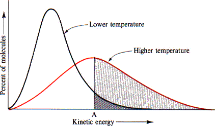
Maxwell-Boltzmann distributions, which we introduced in unit three, describe the distribution of particle energies in samples at different temperatures. They show that as temperature increases, the range of velocities becomes larger, and a fraction of particles move at a higher speed.

A Boltzmann Diagram showing the impact of higher temperatures, Image Courtesy of the University of Illinois at Urbana-Champaign
Effective and Ineffective Collisions
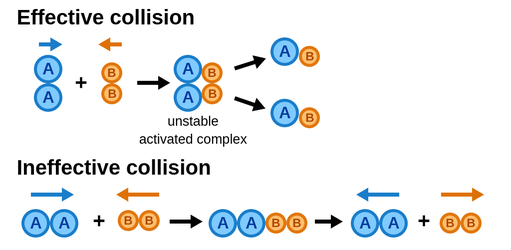
There's one big caveat to the collision model, and that's that not every collision will result in a chemical reaction. This is what separates an effective collision from an ineffective collision. An ineffective collision occurs when there isn't enough force, molecules are moving too slowly, and/or the molecules aren't aligned right. This is why some reactions at different temperatures move at different rates. Here's a picture to help explain:

Image Courtesy of Labster Theory
The biggest takeaway from this study guide is that in most reactions, only a small fraction of the collisions are effective and cause the reaction itself. Effective collisions occur if, and only if, particles have sufficient energy and arrange themselves in the proper orientation.
<< Hide Menu
Dalia Savy
Jacob Jeffries
Dalia Savy
Jacob Jeffries
After plenty of math, we're back to the conceptual part of this unit! Remember that kinetics is the study of the rate of chemical reactions, or basically, how fast a chemical reaction can go. In this study guide, you'll learn that in order for a reaction to proceed, or be successful, very specific conditions must be satisfied.
What is the Collision Model?
The collision model essentially models molecules as projectiles moving in random directions with a fixed average speed that is determined by temperature. As these projectiles collide, they bounce off one another, preserving their kinetic energy and momentum. Thus, through this model, one can see that a reaction is nothing more than two atoms or molecules essentially slamming into each other with:
- enough energy to cause a reaction (the energy needed to cause a reaction is called the activation energy), and
- the correct orientation to form products. This can be seen in the following image:

Image Courtesy of SaylorDotOrg
As we can see in this image, two molecules, nitrogen monoxide and ozone, slam together in an effective collision (we'll see what that means a bit later) to form nitrogen dioxide and molecular oxygen. This reaction serves as an example of what occurs during a chemical reaction according to the kinetic collision model.
The Math Behind the Model
⚠️ You do not need to know this section, but it is worth a read-through to better conceptually understand this model.
An important distinction to recognize is that these collisions are not actually random. Two particles colliding with one another have a very well-defined system of equations that one can use to solve for their trajectories. The first one is the statement about the conservation of kinetic energy:
The second one is the statement of conservation of momentum:
- m1 and m2 both describe the masses of particle 1 and particle 2,
- v1,i and v2,i both describe the initial velocities of particle 1 and 2 before the collision,
- and v1,f, and v2,f both define the final velocities of 1 and 2 after the collision. Qualitatively, Eq. 10 states that the total kinetic energy of the system stays constant, and Eq. 11 states that the total momentum of the system also stays constant.
However, a modification must be made to accurately describe reactive collisions (ie. a collision where a chemical reaction happens), as some of the kinetic energy must be expended to break and create new chemical bonds, thus making the system’s total kinetic energy a non-constant variable.
These equations by themselves are not very useful on a macroscopic scale. These collisions take place within systems of many molecules, and Eq. 10 and Eq. 11 only describe two-particle collisions. At any instant, if we assume each particle collides with another particle at the same time, we would need N/2 systems of equations to describe the system accurately, where N is the number of molecules in the system.
Since each system of equations has two equations, this means one would need (N/2)×2 = N equations to completely model the situation. For the case of a 1.00 mol sample, this number is 6.02 × 10^23. This would be an awful amount of algebra; I would not recommend doing this on paper if you would prefer to keep your fingers attached to your hands.
As such, we must treat the system statistically, meaning we calculate average values instead of individual values. This means we must modify Eq. 10 slightly:
Aavg denotes the average of variable A. We can move the avg subscript to solely the v^2 term because m does not vary throughout the sample (assuming the sample is pure), thus its average is itself. However, this is a measurement of kinetic energy per particle, so we multiply the entire term by N, the number of particles, in order to obtain an expression for the total kinetic energy of the gas:

This is an important equation as it also connects to Eq. 12, which means that, as the average speed of the molecules increases, so does the temperature of the sample and vice versa, since as average velocity increases, total kinetic energy increases. One might be tempted to equate (v2)avg to simply (vavg)^2. There are two reasons why this does not work. For the first example, let's look at three objects traveling at 5.0 m/s, 10 m/s, and 15 m/s. The average speed is:

However,

The second reason is that, in an ideal sample, (vavg)^2 = 0, because the molecules are traveling with random speeds, so the number of molecules traveling to the right is the same as the number traveling leftwards, thus the velocities cancel out, making vavg = 0.
Interpreting the Collision Model
So what can we learn from the collision model about the rate of a chemical reaction? Well first and foremost, we learn that the faster a molecule is moving (and thus the more kinetic energy it has), the more collisions it will make, and therefore the rate of reaction will be faster.
How do we speed up molecules, you may ask? Well, the easiest way to do so is to raise the temperature! The collision model tells us that, in general, when you heat up a reaction it tends to go faster due to more kinetic energy in molecules (this has come up before in FRQs!). This all goes back to the point we keep emphasizing: temperature is the average kinetic energy of particles.
Maxwell-Boltzmann Distributions
Maxwell-Boltzmann distributions, which we introduced in unit three, describe the distribution of particle energies in samples at different temperatures. They show that as temperature increases, the range of velocities becomes larger, and a fraction of particles move at a higher speed.

A Boltzmann Diagram showing the impact of higher temperatures, Image Courtesy of the University of Illinois at Urbana-Champaign
Effective and Ineffective Collisions
There's one big caveat to the collision model, and that's that not every collision will result in a chemical reaction. This is what separates an effective collision from an ineffective collision. An ineffective collision occurs when there isn't enough force, molecules are moving too slowly, and/or the molecules aren't aligned right. This is why some reactions at different temperatures move at different rates. Here's a picture to help explain:

Image Courtesy of Labster Theory
The biggest takeaway from this study guide is that in most reactions, only a small fraction of the collisions are effective and cause the reaction itself. Effective collisions occur if, and only if, particles have sufficient energy and arrange themselves in the proper orientation.

© 2025 Fiveable Inc. All rights reserved.